Las figuras salen de villarrica_45y_diario. El Hovmöller lee esa misma salida, un día de cada 30, y no abre el NetCDF de 3,4 GB de esc_03. La validación contra CTD es la figura 21.
figuras = FileAttachment("../datos/series/gotm_figuras.csv").csv({typed: true})
ranking = FileAttachment("../datos/series/gotm_ranking.csv").csv({typed: true})
hov = FileAttachment("../datos/series/gotm_hov_t.csv").csv({typed: true})

temas = [...new Set(figuras.map(d => d.tema))]
viewof tema = Inputs.select(temas, {label: "Tema", value: "validacion CTD"})
Validación y figuras
{
  const filas = figuras.filter(d => d.tema === tema);
  return html`<div>${filas.map(d => html`<figure>
    <img src="../figs/10-gotm/${d.archivo}" alt="${d.archivo}" style="max-width:100%">
    <figcaption class="portal-origen">${d.ruta}</figcaption>
  </figure>`)}</div>`;
}
Hovmöller de temperatura
Profundidad positiva hacia abajo. Cada celda es un día de la muestra (uno cada 30) y una de las 80 capas.
anio = d => {
  const f = d.fecha;
  if (f instanceof Date) return f.getUTCFullYear();
  return +String(f).slice(0, 4);
}
anios = [...new Set(hov.map(anio))].sort((a, b) => a - b)
viewof desde = Inputs.select(anios, {label: "Desde", value: 2015, format: d => String(d)})
viewof hasta = Inputs.select(anios, {label: "Hasta", value: 2017, format: d => String(d)})
{
  const a = Math.min(desde, hasta);
  const b = Math.max(desde, hasta);
  const filas = hov.filter(d => anio(d) >= a && anio(d) <= b);
  return Plot.plot({
    width: 900,
    height: 460,
    marginLeft: 50,
    color: {scheme: "turbo", legend: true, label: "T [°C]"},
    x: {label: "Fecha"},
    y: {label: "Profundidad [m]", ticks: [1, 40, 80, 120, 165]},
    marks: [
      Plot.cell(filas, {x: "fecha", y: "prof_m", fill: "temp_c", inset: 0})
    ]
  });
}
Origen: 06. GOTM/Datos/Salidas/villarrica_45y_diario.nc, variable temp, un día de cada 30.
Sensibilidad LHS200
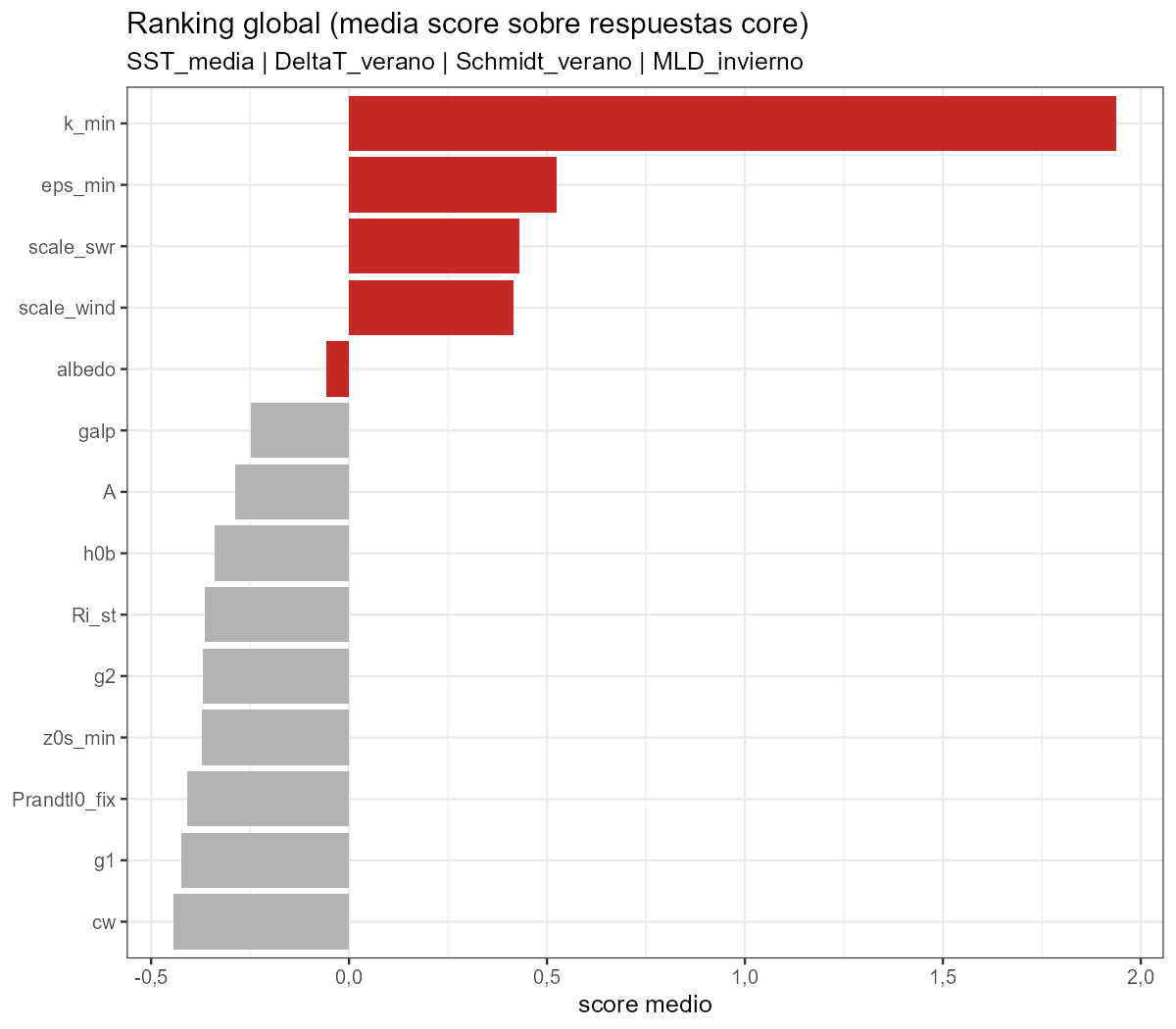
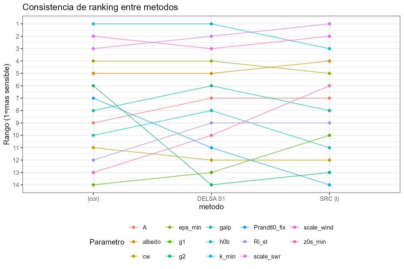
El ranking global promedia el score de SST media, DeltaT de verano, Schmidt de verano y MLD de invierno. El primer puesto es k_min.
Plot.plot({
  width: 720,
  height: 420,
  marginLeft: 90,
  x: {label: "score medio"},
  marks: [
    Plot.barX(ranking, {
      y: "Parametro",
      x: "mean_score",
      fill: d => d.top === true || d.top === "TRUE" ? "#1a5276" : "#b0b8c0",
      sort: {y: "x", reverse: true}
    })
  ]
})
Origen: 09. XLSX/10. GOTM/Sensibilidad_LHS200/02_ranking_DELSA_LHS200.xlsx, hoja RankingGlobal. Las otras PNG de 08. Figs/10. GOTM/Sensibilidad_LHS200/ quedan en esa carpeta.